KV Cache Explained — Why LLMs Eat So Much Memory

If you've ever run an LLM locally, you've seen it: prompts get longer, VRAM usage spikes, and eventually you hit an OOM (Out of Memory) crash. At the center of this memory bottleneck is the KV Cache.

This post covers what the KV Cache is, why it consumes so much memory, and how to calculate the exact memory cost for any model — with code.

Attention in 30 Seconds

The core of every Transformer is Self-Attention. Each token computes its relationship with every other token:

latex

\text{Attention}(Q, K, V) = \text{softmax}\left(\frac{QK^T}{\sqrt{d_k}}\right)V

Each token is projected into three vectors:

Query (Q): "What information do I need?"
Key (K): "What information do I have?"
Value (V): "The actual information to pass along"

The dot product of Q and K determines "which tokens to focus on," and those weights are used to sum the V vectors.

The problem: every token must compute its relation to all previous tokens. For sequence length $n$, compute scales as $O(n^2)$.

Why the KV Cache Exists

LLMs generate tokens one at a time, sequentially. When generating the next token after a prompt, the model needs the Key and Value vectors of all previous tokens.

Without the KV Cache:

Generate token 1: Compute K, V for the entire prompt
Generate token 2: Recompute K, V for prompt + token 1 from scratch
Generate token 3: Recompute everything again...

This is massively wasteful. The KV Cache stores previously computed K and V vectors in memory so they never need to be recomputed.

[Without KV Cache]
Token 1: Compute K,V → 4 tokens
Token 2: Compute K,V → 5 tokens (all recomputed)
Token 3: Compute K,V → 6 tokens (all recomputed)
→ Total ops: 4 + 5 + 6 = 15

[With KV Cache]
Token 1: Compute K,V → 4 tokens (store in cache)
Token 2: Compute K,V → 1 new token + reuse cache
Token 3: Compute K,V → 1 new token + reuse cache
→ Total ops: 4 + 1 + 1 = 6

Compute drops dramatically, but cache memory grows linearly with sequence length.

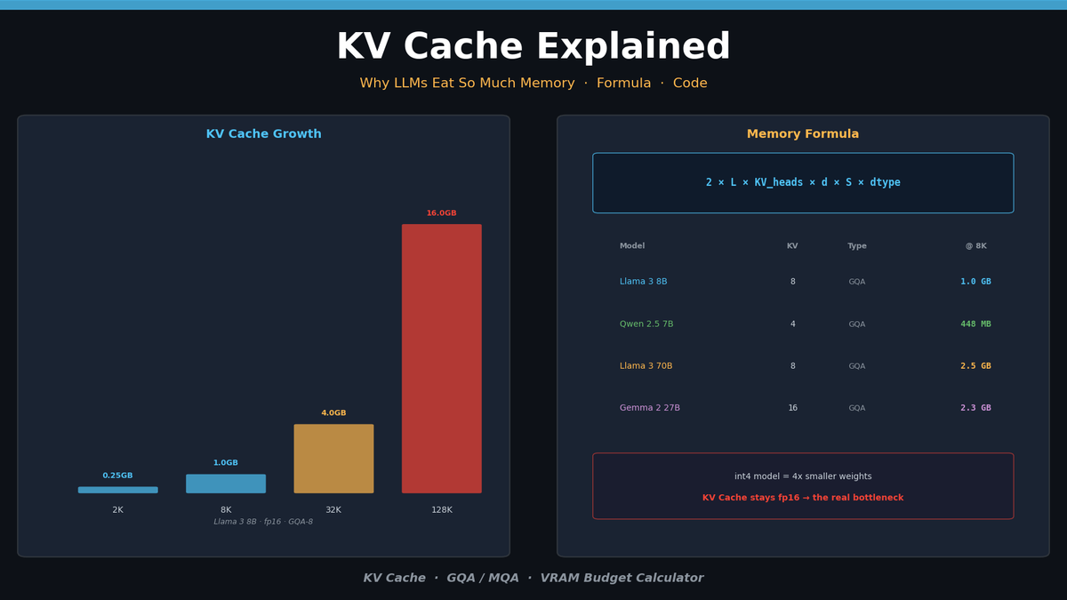
KV Cache Memory Formula

The memory footprint can be calculated precisely:

latex

\text{KV Cache} = 2 \times L \times n_{kv} \times d_{head} \times S \times b

Variable	Meaning	Example
$2$	Key and Value	Fixed
$L$	Number of Transformer layers	32 (Llama 3 8B)
$n_{kv}$	Number of KV heads	8 (GQA), 32 (MHA)
$d_{head}$	Head dimension	128
$S$	Sequence length	8,192
$b$	Bytes per element	2 (fp16), 1 (int8)

The critical variable is $n_{kv}$. Traditional Multi-Head Attention (MHA) uses equal numbers of Query and KV heads. Modern models use GQA (Grouped-Query Attention) to dramatically reduce the KV head count.

KV Cache Size by Model

Here's the actual KV Cache memory for popular models at 8K sequence length in fp16:

Model	Layers	KV Heads	Head Dim	Attention	Per Token	@ 8K	@ 128K
Llama 3 8B	32	8	128	GQA	128 KB	1.0 GB	16 GB
Llama 3 70B	80	8	128	GQA	320 KB	2.5 GB	40 GB
Qwen 2.5 7B	28	4	128	GQA	56 KB	448 MB	7 GB
Mistral 7B	32	8	128	GQA	128 KB	1.0 GB	16 GB
Gemma 2 27B	46	16	128	GQA	288 KB	2.3 GB	36 GB

Even at the same parameter count, the number of GQA KV heads completely changes cache size. Qwen 2.5 7B uses only 4 KV heads — less than half the cache memory of Llama 3 8B.

At 128K context, Llama 3 70B's KV Cache alone is 40 GB — on top of the 140 GB model weights (fp16).

Hands-On: Inspecting KV Cache in Python

Checking KV Cache Shape

python

from transformers import AutoModelForCausalLM, AutoTokenizer
import torch

model_id = "Qwen/Qwen2.5-7B-Instruct"
tokenizer = AutoTokenizer.from_pretrained(model_id)
model = AutoModelForCausalLM.from_pretrained(
    model_id,
    torch_dtype=torch.float16,
    device_map="auto",
)

# Tokenize prompt
prompt = "Explain the KV cache in transformers."
inputs = tokenizer(prompt, return_tensors="pt").to(model.device)

# Get KV Cache with use_cache=True
with torch.no_grad():
    outputs = model(**inputs, use_cache=True)

# Inspect KV Cache structure
past_kv = outputs.past_key_values
print(f"Layers: {len(past_kv)}")
print(f"Key shape: {past_kv[0][0].shape}")  # (batch, kv_heads, seq_len, head_dim)
print(f"Value shape: {past_kv[0][1].shape}")

# Calculate total KV Cache memory
total_bytes = sum(
    k.element_size() * k.nelement() + v.element_size() * v.nelement()
    for k, v in past_kv
)
print(f"KV Cache memory: {total_bytes / 1024**2:.1f} MB")

Example output (Qwen 2.5 7B, 8-token prompt):

Layers: 28
Key shape: torch.Size([1, 4, 8, 128])
Value shape: torch.Size([1, 4, 8, 128])
KV Cache memory: 0.4 MB

Memory Profiling by Context Length

python

import torch
import matplotlib.pyplot as plt

def measure_kv_cache_memory(model, tokenizer, seq_lengths):
    """Measure KV Cache memory at different sequence lengths"""
    results = []

    for length in seq_lengths:
        input_ids = torch.randint(
            100, 30000, (1, length), device=model.device
        )

        torch.cuda.empty_cache()
        torch.cuda.reset_peak_memory_stats()

        with torch.no_grad():
            outputs = model(input_ids, use_cache=True)

        past_kv = outputs.past_key_values
        kv_bytes = sum(
            k.element_size() * k.nelement() + v.element_size() * v.nelement()
            for k, v in past_kv
        )

        results.append({
            'seq_len': length,
            'kv_cache_mb': kv_bytes / 1024**2,
            'total_gpu_mb': torch.cuda.max_memory_allocated() / 1024**2,
        })

        del outputs, past_kv
        torch.cuda.empty_cache()

    return results

# Measure
seq_lengths = [512, 1024, 2048, 4096, 8192, 16384]
results = measure_kv_cache_memory(model, tokenizer, seq_lengths)

# Visualize
fig, (ax1, ax2) = plt.subplots(1, 2, figsize=(14, 5))

lengths = [r['seq_len'] for r in results]
kv_sizes = [r['kv_cache_mb'] for r in results]
total_sizes = [r['total_gpu_mb'] for r in results]

ax1.plot(lengths, kv_sizes, 'o-', color='#4FC3F7', linewidth=2, markersize=8)
ax1.set_xlabel('Sequence Length')
ax1.set_ylabel('KV Cache (MB)')
ax1.set_title('KV Cache Memory vs Sequence Length')
ax1.grid(True, alpha=0.3)

kv_ratio = [kv / total * 100 for kv, total in zip(kv_sizes, total_sizes)]
ax2.bar(range(len(lengths)), kv_ratio, color='#FFB74D', alpha=0.8)
ax2.set_xticks(range(len(lengths)))
ax2.set_xticklabels([f'{l//1024}K' for l in lengths])
ax2.set_ylabel('KV Cache / Total GPU Memory (%)')
ax2.set_title('KV Cache Ratio in Total GPU Usage')
ax2.grid(True, alpha=0.3, axis='y')

plt.tight_layout()
plt.savefig('kv_cache_profile.png', dpi=150, bbox_inches='tight')
plt.show()

Running this code produces a perfectly linear graph — KV Cache memory scales exactly with sequence length. As context grows longer, the KV Cache's share of total GPU memory steadily increases.

GQA / MQA — The Key to Smaller KV Caches

The biggest lever for KV Cache size is the number of KV heads. This varies by attention type.

Multi-Head Attention (MHA)

The original Transformer design. Query, Key, and Value all have the same number of heads.

Q Heads: [H0] [H1] [H2] [H3] [H4] [H5] [H6] [H7]
K Heads: [H0] [H1] [H2] [H3] [H4] [H5] [H6] [H7]
V Heads: [H0] [H1] [H2] [H3] [H4] [H5] [H6] [H7]
→ KV Cache: 8 × head_dim × 2 per token per layer

Grouped-Query Attention (GQA)

Multiple Query heads share a single KV head. Used by Llama 3, Qwen 2.5, and most modern models.

Q Heads: [H0] [H1] [H2] [H3] [H4] [H5] [H6] [H7]
K Heads: [K0      ] [K1      ] [K2      ] [K3      ]
V Heads: [V0      ] [V1      ] [V2      ] [V3      ]
→ KV Cache: 4 × head_dim × 2 per token per layer (half!)

Multi-Query Attention (MQA)

All Query heads share a single KV head. Most aggressive compression, but can hurt quality.

Q Heads: [H0] [H1] [H2] [H3] [H4] [H5] [H6] [H7]
K Heads: [K0                                      ]
V Heads: [V0                                      ]
→ KV Cache: 1 × head_dim × 2 per token per layer (1/8!)

Checking in Code

python

from transformers import AutoConfig

models = [
    "meta-llama/Llama-3.1-8B-Instruct",
    "Qwen/Qwen2.5-7B-Instruct",
    "mistralai/Mistral-7B-Instruct-v0.3",
    "google/gemma-2-9b-it",
]

print(f"{'Model':<40} {'Layers':>7} {'Q Heads':>8} {'KV Heads':>9} {'Head Dim':>9} {'Type':>5}")
print("-" * 80)

for model_id in models:
    config = AutoConfig.from_pretrained(model_id)
    q_heads = config.num_attention_heads
    kv_heads = getattr(config, 'num_key_value_heads', q_heads)
    head_dim = config.hidden_size // q_heads

    if kv_heads == q_heads:
        attn_type = "MHA"
    elif kv_heads == 1:
        attn_type = "MQA"
    else:
        attn_type = "GQA"

    print(f"{model_id:<40} {config.num_hidden_layers:>7} {q_heads:>8} {kv_heads:>9} {head_dim:>9} {attn_type:>5}")

Practical: Calculating Your VRAM Budget

The most important question for deployment: "Will this model fit on my GPU?"

Total VRAM = Model Weights + KV Cache + Overhead

python

def calculate_vram_budget(
    model_params_b: float,  # Model parameters (billions)
    num_layers: int,
    kv_heads: int,
    head_dim: int,
    max_seq_len: int,
    batch_size: int = 1,
    model_dtype_bytes: int = 2,  # fp16=2, int4=0.5
    kv_dtype_bytes: int = 2,     # fp16=2, int8=1
):
    """Calculate VRAM usage in GB"""

    # 1. Model weights
    model_memory_gb = model_params_b * 1e9 * model_dtype_bytes / 1024**3

    # 2. KV Cache
    kv_cache_bytes = (
        2  # K + V
        * num_layers
        * kv_heads
        * head_dim
        * max_seq_len
        * batch_size
        * kv_dtype_bytes
    )
    kv_cache_gb = kv_cache_bytes / 1024**3

    # 3. Overhead (activations, CUDA context, etc.) — ~10-20%
    overhead_gb = (model_memory_gb + kv_cache_gb) * 0.15

    total_gb = model_memory_gb + kv_cache_gb + overhead_gb

    return {
        'model_weights_gb': round(model_memory_gb, 1),
        'kv_cache_gb': round(kv_cache_gb, 1),
        'overhead_gb': round(overhead_gb, 1),
        'total_gb': round(total_gb, 1),
    }

# Example: Llama 3 8B (fp16) + 8K context
result = calculate_vram_budget(
    model_params_b=8,
    num_layers=32,
    kv_heads=8,
    head_dim=128,
    max_seq_len=8192,
)
print("Llama 3 8B @ 8K context (fp16):")
for k, v in result.items():
    print(f"  {k}: {v} GB")

# Example: Llama 3 8B (int4 quantized) + 32K context
result_q = calculate_vram_budget(
    model_params_b=8,
    num_layers=32,
    kv_heads=8,
    head_dim=128,
    max_seq_len=32768,
    model_dtype_bytes=0.5,  # int4
    kv_dtype_bytes=2,       # KV still fp16
)
print("\nLlama 3 8B (int4) @ 32K context:")
for k, v in result_q.items():
    print(f"  {k}: {v} GB")

Example output:

Llama 3 8B @ 8K context (fp16):
  model_weights_gb: 14.9
  kv_cache_gb: 1.0
  overhead_gb: 2.4
  total_gb: 18.3

Llama 3 8B (int4) @ 32K context:
  model_weights_gb: 3.7
  kv_cache_gb: 4.0
  overhead_gb: 1.2
  total_gb: 8.9

Here's the key insight: int4 quantization shrinks model weights by 4x, but the KV Cache remains fp16. At longer contexts, the KV Cache can consume more VRAM than the model weights themselves.

This is exactly why KV Cache optimization matters.

KV Cache Optimization Approaches

There are three main directions for tackling KV Cache memory:

1. KV Cache Quantization: Compress the cache from fp16 → int8/int4. Cuts memory 2-4x but introduces precision loss.

2. Sparse Attention: Attend to only the most important tokens instead of all tokens. DeepSeek's DSA and Nvidia's DMS are leading examples.

3. KV Cache Compression: Mathematically compress the cache data itself using techniques like PCA. Nvidia's KVTC achieves up to 20x compression.

Premium Series4 parts

LLM Inference Optimization Series — From Attention to Production Serving

Parts 1-4 cover Attention internals, KV Cache optimization, Sparse Attention, and vLLM/TGI production deployment with hands-on code.

View Series →Compare plans

Summary

Topic	Key Takeaway
What is KV Cache	Stores previous tokens' Key/Value vectors to avoid recomputation
Size factors	Layers × KV Heads × Head Dim × Sequence Length
Role of GQA	Reduces KV heads to cut cache memory by 2-8x
Practical note	Quantized models still use fp16 KV Cache — bottleneck at long contexts

The KV Cache is the central bottleneck of LLM inference. From model selection to serving architecture, how efficiently you manage this memory determines both performance and cost.

KV Cache Explained — Why LLMs Eat So Much Memory